Machine learning (ML) powered anomaly detection

Overview

As of v1.32.0, Netdata comes with some ML powered anomaly detection capabilities built into it and available to use out of the box, with minimal configuration required.

🚧 Note: This functionality is still under active development and considered experimental. Changes might cause the feature to break. We dogfood it internally and among early adopters within the Netdata community to build the feature. If you would like to get involved and help us with some feedback, email us at analytics-ml-team@netdata.cloud, comment on the beta launch post in the Netdata community, or come join us in the 🤖-ml-powered-monitoring channel of the Netdata discord.

Once ML is enabled, Netdata will begin training a model for each dimension. By default this model is a k-means clustering model trained on the most recent 4 hours of data. Rather than just using the most recent value of each raw metric, the model works on a preprocessed "feature vector" of recent smoothed and differenced values. This should enable the model to detect a wider range of potentially anomalous patterns in recent observations as opposed to just point anomalies like big spikes or drops. (This infographic shows some different types of anomalies.)

The sections below will introduce some of the main concepts:

• anomaly bit
• anomaly score
• anomaly rate
• anomaly detector

Additional explanations and details can be found in the Glossary and Notes at the bottom of the page.

Anomaly Bit - (100 = Anomalous, 0 = Normal)

Once each model is trained, Netdata will begin producing an "anomaly score" at each time step for each dimension. This "anomaly score" is essentially a distance measure to the trained cluster centers of the model (by default each model has k=2, so two cluster centers are learned). More anomalous looking data should be more distant to those cluster centers. If this "anomaly score" is sufficiently large, this is a sign that the recent raw values of the dimension could potentially be anomalous. By default, "sufficiently large" means that the distance is in the 99th percentile or above of all distances observed during training or, put another way, it has to be further away than the furthest 1% of the data used during training. Once this threshold is passed, the "anomaly bit" corresponding to that dimension is set to 100 to flag it as anomalous, otherwise it would be left at 0 to signal normal data.

What this means is that in addition to the raw value of each metric, Netdata now also stores an "anomaly bit" that is either 100 (anomalous) or 0 (normal). Importantly, this is achieved without additional storage overhead due to how the anomaly bit has been implemented within the existing internal Netdata storage representation.

This "anomaly bit" is exposed via the anomaly-bit key that can be passed to the options param of the /api/v1/data REST API.

For example, here are some recent raw dimension values for system.ip on our london demo server:

https://london.my-netdata.io/api/v1/data?chart=system.ip

{
 "labels": ["time", "received", "sent"],
    "data":
 [
      [ 1638365672, 54.84098, -76.70201],
      [ 1638365671, 124.4328, -309.7543],
      [ 1638365670, 123.73152, -167.9056],
      ...
 ]
}

And if we add the &options=anomaly-bit params, we can see the "anomaly bit" value corresponding to each raw dimension value:

https://london.my-netdata.io/api/v1/data?chart=system.ip&options=anomaly-bit

{
 "labels": ["time", "received", "sent"],
    "data":
 [
      [ 1638365672, 0, 0],
      [ 1638365671, 0, 0],
      [ 1638365670, 0, 0],
      ...
 ]
}

In this example, the dimensions "received" and "sent" didn't show any abnormal behavior, so the anomaly bit is zero. Under normal circumstances, the anomaly bit will mostly be 0. However, there can be random fluctuations setting the anomaly to 100, although this very much depends on the nature of the dimension in question.

Anomaly Rate - average(anomaly bit)

Once all models have been trained, we can think of the Netdata dashboard as essentially a big matrix or table of 0's and 100's. If we consider this "anomaly bit"-based representation of the state of the node, we can now think about how we might detect overall node level anomalies. The figure below illustrates the main ideas.

        dimensions
time    d1  d2  d3  d4  d5      NAR
   1    0   0   0   0   0        0%
   2    0   0   0   0   100     20%
   3    0   0   0   0   0        0%
   4    0   100 0   0   0       20%
   5    100 0   0   0   0       20%
   6    0   100 100 0   100     60%
   7    0   100 0   100 0       40%
   8    0   0   0   0   100     20%
   9    0   0   100 100 0       40%
   10   0   0   0   0   0        0%
 
DAR     10% 30% 20% 20% 30%     22% NAR_t1-t10

DAR        = Dimension Anomaly Rate
NAR        = Node Anomaly Rate
NAR_t1-t10 = Node Anomaly Rate over t1 to t10

To work out an "anomaly rate", we can just average a row or a column in any direction. For example, if we were to just average along a row then this would be the "node anomaly rate" (all dimensions) at time t. Likewise if we averaged a column then we would have the "dimension anomaly rate" for each dimension over the time window t=1-10. Extending this idea, we can work out an overall "anomaly rate" for the whole matrix or any subset of it we might be interested in.

Anomaly Detector - Node level anomaly events

An "anomaly detector" looks at all anomaly bits of a node. Netdata's anomaly detector produces an "anomaly event" when a the percentage of anomaly bits is high enough for a persistent amount of time. This anomaly event signals that there was sufficient evidence among all the anomaly bits that some strange behavior might have been detected in a more global sense across the node.

Essentially if the "Node Anomaly Rate" (NAR) passes a defined threshold and stays above that threshold for a persistent amount of time, a "Node Anomaly Event" will be triggered.

These anomaly events are currently exposed via /api/v1/anomaly_events

Note: Clicking the link below will likely return an empty list of []. This is the response when no anomaly events exist in the specified range. The example response below is illustrative of what the response would be when one or more anomaly events exist within the range of after to before.

https://london.my-netdata.io/api/v1/anomaly_events?after=1638365182000&before=1638365602000

If an event exists within the window, the result would be a list of start and end times.

[
    [
        1638367788,
        1638367851
    ]
]

Information about each anomaly event can then be found at the /api/v1/anomaly_event_info endpoint (making sure to pass the after and before params):

Note: If you click the below url you will get a null since no such anomaly event exists as the response is just an illustrative example taken from a node that did have such an anomaly event.

https://london.my-netdata.io/api/v1/anomaly_event_info?after=1638367788&before=1638367851

[
    [
        0.66,
        "netdata.response_time|max"
    ],
    [
        0.63,
        "netdata.response_time|average"
    ],
    [
        0.54,
        "netdata.requests|requests"
    ],
    ...

The query returns a list of dimension anomaly rates for all dimensions that were considered part of the detected anomaly event.

Note: We plan to build additional anomaly detection and exploration features into both Netdata Agent and Netdata Cloud. The current endpoints are still under active development to power the upcoming features.

Configuration

To enable anomaly detection:

1. Find and open the Netdata configuration file netdata.conf.
2. In the [ml] section, set enabled = yes.
3. Restart netdata (typically sudo systemctl restart netdata).

Note: If you would like to learn more about configuring Netdata please see the configuration guide.

Below is a list of all the available configuration params and their default values.

[ml]
    # enabled = no
    # maximum num samples to train = 14400
    # minimum num samples to train = 3600
    # train every = 3600
    # dbengine anomaly rate every = 60
    # num samples to diff = 1
    # num samples to smooth = 3
    # num samples to lag = 5
    # random sampling ratio = 0.2
    # maximum number of k-means iterations = 1000
    # dimension anomaly score threshold = 0.99
    # host anomaly rate threshold = 0.01000
    # minimum window size = 30.00000
    # maximum window size = 600.00000
    # idle window size = 30.00000
    # window minimum anomaly rate = 0.25000
    # anomaly event min dimension rate threshold = 0.05000
    # hosts to skip from training = !*
    # charts to skip from training = netdata.*

Configuration Examples

If you would like to run ML on a parent instead of at the edge, some configuration options are illustrated below.

This example assumes 3 child nodes streaming to 1 parent node and illustrates the main ways you might want to configure running ml for the children on the parent, running ML on the children themselves, or even a mix of approaches.

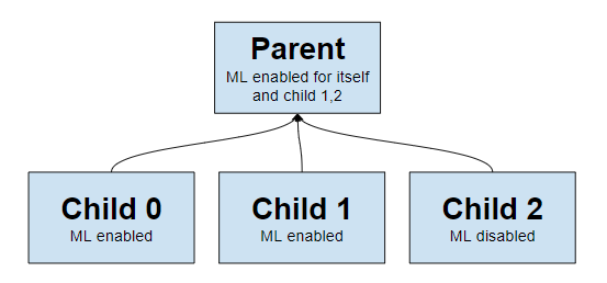
# parent will run ml for itself and child 1,2.
# child 0 will run its own ml at the edge and just stream its ml charts to parent.
# child 1 will run its own ml at the edge, even though parent will also run ml for it, a bit wasteful potentially to run ml in both places but is possible.
# child 2 will not run ml at the edge, it will be run in the parent only.

# parent-ml-ml-stress-0
# run ml on all hosts apart from child-ml-ml-stress-0
[ml]
        enabled = yes
        minimum num samples to train = 900
        train every = 900
        charts to skip from training = !*
        hosts to skip from training = child-ml-ml-stress-0

# child-ml-ml-stress-0
# run ml on child-ml-ml-stress-0 and stream ml charts to parent
[ml]
        enabled = yes
        minimum num samples to train = 900
        train every = 900
        stream anomaly detection charts = yes

# child-ml-ml-stress-1
# run ml on child-ml-ml-stress-1 and stream ml charts to parent
[ml]
        enabled = yes
        minimum num samples to train = 900
        train every = 900
        stream anomaly detection charts = yes

# child-ml-ml-stress-2
# don't run ml on child-ml-ml-stress-2, it will instead run on parent-ml-ml-stress-0
[ml]
        enabled = no

Descriptions (min/max)

• enabled: yes to enable, no to disable.
• maximum num samples to train: (3600/21600) This is the maximum amount of time you would like to train each model on. For example, the default of 14400 trains on the preceding 4 hours of data, assuming an update every of 1 second.
• minimum num samples to train: (900/21600) This is the minimum amount of data required to be able to train a model. For example, the default of 3600 implies that once at least 1 hour of data is available for training, a model is trained, otherwise it is skipped and checked again at the next training run.
• train every: (1800/21600) This is how often each model will be retrained. For example, the default of 3600 means that each model is retrained every hour. Note: The training of all models is spread out across the train every period for efficiency, so in reality, it means that each model will be trained in a staggered manner within each train every period.
• dbengine anomaly rate every: (30/900) This is how often netdata will aggregate all the anomaly bits into a single chart (anomaly_detection.anomaly_rates). The aggregation into a single chart allows enabling anomaly rate ranking over all metrics with one API call as opposed to a call per chart.
• num samples to diff: (0/1) This is a 0 or 1 to determine if you want the model to operate on differences of the raw data or just the raw data. For example, the default of 1 means that we take differences of the raw values. Using differences is more general and works on dimensions that might naturally tend to have some trends or cycles in them that is normal behavior to which we don't want to be too sensitive.
• num samples to smooth: (0/5) This is a small integer that controls the amount of smoothing applied as part of the feature processing used by the model. For example, the default of 3 means that the rolling average of the last 3 values is used. Smoothing like this helps the model be a little more robust to spiky types of dimensions that naturally "jump" up or down as part of their normal behavior.
• num samples to lag: (0/5) This is a small integer that determines how many lagged values of the dimension to include in the feature vector. For example, the default of 5 means that in addition to the most recent (by default, differenced and smoothed) value of the dimension, the feature vector will also include the 5 previous values too. Using lagged values in our feature representation allows the model to work over strange patterns over recent values of a dimension as opposed to just focusing on if the most recent value itself is big or small enough to be anomalous.
• random sampling ratio: (0.2/1.0) This parameter determines how much of the available training data is randomly sampled when training a model. The default of 0.2 means that Netdata will train on a random 20% of training data. This parameter influences cost efficiency. At 0.2 the model is still reasonably trained while minimizing system overhead costs caused by the training.
• maximum number of k-means iterations: This is a parameter that can be passed to the model to limit the number of iterations in training the k-means model. Vast majority of cases can ignore and leave as default.
• dimension anomaly score threshold: (0.01/5.00) This is the threshold at which an individual dimension at a specific timestep is considered anomalous or not. For example, the default of 0.99 means that a dimension with an anomaly score of 99% or higher is flagged as anomalous. This is a normalized probability based on the training data, so the default of 99% means that anything that is as strange (based on distance measure) or more strange as the most strange 1% of data observed during training will be flagged as anomalous. If you wanted to make the anomaly detection on individual dimensions more sensitive you could try a value like 0.90 (90%) or to make it less sensitive you could try 1.5 (150%).
• host anomaly rate threshold: (0.0/1.0) This is the percentage of dimensions (based on all those enabled for anomaly detection) that need to be considered anomalous at specific timestep for the host itself to be considered anomalous. For example, the default value of 0.01 means that if more than 1% of dimensions are anomalous at the same time then the host itself is considered in an anomalous state.
• minimum window size: The Netdata "Anomaly Detector" logic works over a rolling window of data. This parameter defines the minimum length of window to consider. If over this window the host is in an anomalous state then an anomaly detection event will be triggered. For example, the default of 30 means that the detector will initially work over a rolling window of 30 seconds. Note: The length of this window will be dynamic once an anomaly event has been triggered such that it will expand as needed until either the max length of an anomaly event is hit or the host settles back into a normal state with sufficiently decreased host level anomaly states in the rolling window. Note: If you wanted to adjust the higher level anomaly detector behavior then this is one parameter you might adjust to see the impact of on anomaly detection events.
• maximum window size: This parameter defines the maximum length of window to consider. If an anomaly event reaches this size, it will be closed. This is to provide an upper bound on the length of an anomaly event and cost of the anomaly detector logic for that event.
• window minimum anomaly rate: (0.0/1.0) This parameter corresponds to a threshold on the percentage of time in the rolling window that the host was considered in an anomalous state. For example, the default of 0.25 means that if the host is in an anomalous state for 25% of more of the rolling window then and anomaly event will be triggered or extended if one is already active. Note: If you want to make the anomaly detector itself less sensitive, you can adjust this value to something like 0.75 which would mean the host needs to be much more consistently in an anomalous state to trigger an anomaly detection event. Likewise, a lower value like 0.1 would make the anomaly detector more sensitive.
• anomaly event min dimension rate threshold: (0.0/1.0) This is a parameter that helps filter out irrelevant dimensions from anomaly events. For example, the default of 0.05 means that only dimensions that were considered anomalous for at least 5% of the anomaly event itself will be included in that anomaly event. The idea here is to just include dimensions that were consistently anomalous as opposed to those that may have just randomly happened to be anomalous at the same time.
• hosts to skip from training: This parameter allows you to turn off anomaly detection for any child hosts on a parent host by defining those you would like to skip from training here. For example, a value like dev-* skips all hosts on a parent that begin with the "dev-" prefix. The default value of !* means "don't skip any".
• charts to skip from training: This parameter allows you to exclude certain charts from anomaly detection. By default, only netdata related charts are excluded. This is to avoid the scenario where accessing the netdata dashboard could itself tigger some anomalies if you don't access them regularly. If you want to include charts that are excluded by default, add them in small groups and then measure any impact on performance before adding additional ones. Example: If you want to include system, apps, and user charts:!system.* !apps.* !user.* *.

Charts

Once enabled, the "Anomaly Detection" menu and charts will be available on the dashboard.

In terms of anomaly detection, the most interesting charts would be the anomaly_detection.dimensions and anomaly_detection.anomaly_rate ones, which hold the anomalous and anomaly_rate dimensions that show the overall number of dimensions considered anomalous at any time and the corresponding anomaly rate.

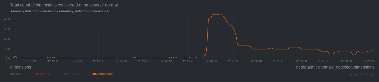
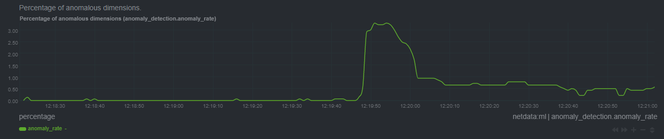
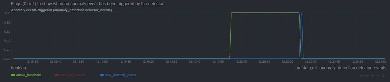
• anomaly_detection.dimensions: Total count of dimensions considered anomalous or normal.
• anomaly_detection.dimensions: Percentage of anomalous dimensions.
• anomaly_detection.detector_window: The length of the active window used by the detector.
• anomaly_detection.detector_events: Flags (0 or 1) to show when an anomaly event has been triggered by the detector.
• anomaly_detection.prediction_stats: Diagnostic metrics relating to prediction time of anomaly detection.
• anomaly_detection.training_stats: Diagnostic metrics relating to training time of anomaly detection.

Below is an example of how these charts may look in the presence of an anomaly event.

Initially we see a jump in anomalous dimensions:

And a corresponding jump in the anomaly_rate:

After a short while the rolling node anomaly rate goes above_threshold, and once it stays above threshold for long enough a new_anomaly_event is created:

Glossary

feature vector

A feature vector is what the ML model is trained on and uses for prediction. The most simple feature vector would be just the latest raw dimension value itself [x]. By default Netdata will use a feature vector consisting of the 6 latest differences and smoothed values of the dimension so conceptually something like [avg3(diff1(x-5)), avg3(diff1(x-4)), avg3(diff1(x-3)), avg3(diff1(x-2)), avg3(diff1(x-1)), avg3(diff1(x))] which ends up being just 6 floating point numbers that try and represent the "shape" of recent data.

anomaly score

At prediction time the anomaly score is just the distance of the most recent feature vector to the trained cluster centers of the model, which are themselves just feature vectors, albeit supposedly the best most representative feature vectors that could be "learned" from the training data. So if the most recent feature vector is very far away in terms of euclidean distance it's more likely that the recent data it represents consists of some strange pattern not commonly found in the training data.

anomaly bit

If the anomaly score is greater than a specified threshold then the most recent feature vector, and hence most recent raw data, is considered anomalous. Since storing the raw anomaly score would essentially double amount of storage space Netdata would need, we instead efficiently store just the anomaly bit in the existing internal Netdata data representation without any additional storage overhead.

anomaly rate

An anomaly rate is really just an average over one or more anomaly bits. An anomaly rate can be calculated over time for one or more dimensions or at a point in time across multiple dimensions, or some combination of the two. Its just an average of some collection of anomaly bits.

anomaly detector

The is essentially business logic that just tries to process a collection of anomaly bits to determine if there is enough active anomaly bits to merit investigation or declaration of a node level anomaly event.

anomaly event

Anomaly events are triggered by the anomaly detector and represent a window of time on the node with sufficiently elevated anomaly rates across all dimensions.

dimension anomaly rate

The anomaly rate of a specific dimension over some window of time.

node anomaly rate

The anomaly rate across all dimensions of a node.

Notes

• We would love to hear any feedback relating to this functionality, please email us at analytics-ml-team@netdata.cloud or come join us in the 🤖-ml-powered-monitoring channel of the Netdata discord.
• We are working on additional UI/UX based features that build on these core components to make them as useful as possible out of the box.
• Although not yet a core focus of this work, users could leverage the anomaly_detection chart dimensions and/or anomaly-bit options in defining alarms based on ML driven anomaly detection models.
• This presentation walks through some of the main concepts covered above in a more informal way.
• After restart Netdata will wait until minimum num samples to train observations of data are available before starting training and prediction.
• Netdata uses dlib under the hood for its core ML features.
• You should benchmark Netdata resource usage before and after enabling ML. Typical overhead ranges from 1-2% additional CPU at most.
• The "anomaly bit" has been implemented to be a building block to underpin many more ML based use cases that we plan to deliver soon.
• At its core Netdata uses an approach and problem formulation very similar to the Netdata python anomalies collector, just implemented in a much much more efficient and scalable way in the agent in c++. So if you would like to learn more about the approach and are familiar with Python that is a useful resource to explore, as is the corresponding deep dive tutorial where the default model used is PCA instead of K-Means but the overall approach and formulation is similar.